Calculate Wald-Profiles

Transforms a signed root deviance profile of a mcprofile object into a profile of Wald-type statistics

wald(object)

Arguments

object	An object of class mcprofile

Value

An object of class mcprofile with a wald profile in the srdp slot.

See also

mcprofile

Examples

#######################################
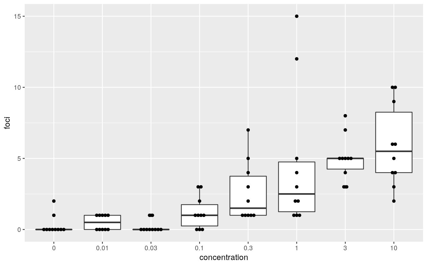
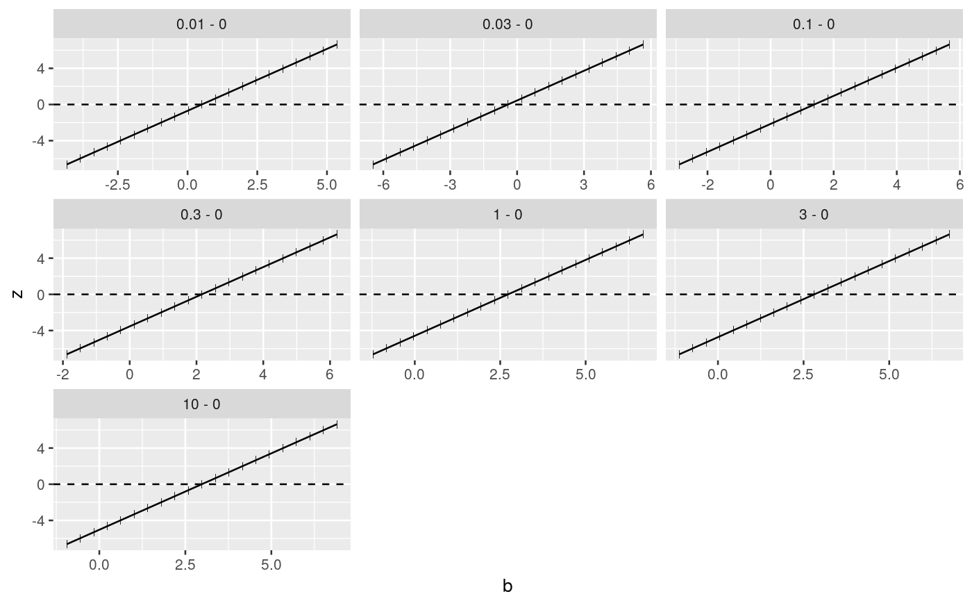
## cell transformation assay example ##
#######################################

str(cta)
#> 'data.frame':	80 obs. of  2 variables:
#>  $ conc: num  0 0 0 0 0 0 0 0 0 0 ...
#>  $ foci: int  0 1 0 0 0 0 0 0 0 2 ...
## change class of cta$conc into factor
cta$concf <- factor(cta$conc, levels=unique(cta$conc))

ggplot(cta, aes(y=foci, x=concf)) +
  geom_boxplot() +
  geom_dotplot(binaxis = "y", stackdir = "center", binwidth = 0.2) +
  xlab("concentration")


# glm fit assuming a Poisson distribution for foci counts
# parameter estimation on the log link
# removing the intercept
fm <- glm(foci ~ concf-1, data=cta, family=poisson(link="log"))

### Comparing each dose to the control by Dunnett-type comparisons
# Constructing contrast matrix
library(multcomp)
CM <- contrMat(table(cta$concf), type="Dunnett")

# calculating signed root deviance profiles
(dmcp <- mcprofile(fm, CM))
#> 
#>    Multiple Contrast Profiles
#> 
#>          Estimate Std.err
#> 0.01 - 0    0.511   0.730
#> 0.03 - 0   -0.405   0.913
#> 0.1 - 0     1.386   0.645
#> 0.3 - 0     2.159   0.610
#> 1 - 0       2.730   0.596
#> 3 - 0       2.813   0.594
#> 10 - 0      2.979   0.592
#> 
# computing profiles for the modified likelihood root
wp <- wald(dmcp)

plot(wp)

# comparing confidence intervals
confint(wp)
#> 
#>    mcprofile - Confidence Intervals 
#> 
#> level: 		 0.95 
#> adjustment:	 single-step 
#> 
#>          Estimate  lower upper
#> 0.01 - 0    0.511 -1.269  2.29
#> 0.03 - 0   -0.405 -2.630  1.82
#> 0.1 - 0     1.386 -0.187  2.96
#> 0.3 - 0     2.159  0.673  3.65
#> 1 - 0       2.730  1.278  4.18
#> 3 - 0       2.813  1.365  4.26
#> 10 - 0      2.979  1.536  4.42
#> 
confint(dmcp)
#> 
#>    mcprofile - Confidence Intervals 
#> 
#> level: 		 0.95 
#> adjustment:	 single-step 
#> 
#>          Estimate   lower upper
#> 0.01 - 0    0.511 -1.2495  2.56
#> 0.03 - 0   -0.405 -3.0528  1.87
#> 0.1 - 0     1.386 -0.0177  3.31
#> 0.3 - 0     2.159  0.8957  4.04
#> 1 - 0       2.730  1.5191  4.59
#> 3 - 0       2.813  1.6080  4.67
#> 10 - 0      2.979  1.7832  4.83
#>