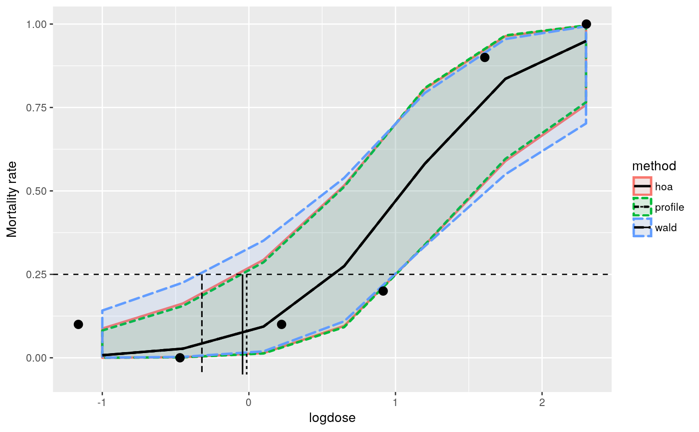
Identifying the lethal dose of a crop protection product.

Increasing dose levels of a toxin, used as a pesticide for crop protection, is applied to non-target species. The lethal dose should be identified in this experiment. The dataset represents simulated data based on a real experiment.

toxinLD

Format

A data frame with 6 observations on the following 3 variables.

dose

a numeric vector denoting the toxin concentration levels

dead

a numeric vector with the number of dead insects.

alive

a numeric vector with the number of surviving insects.

Examples

str(toxinLD)
#> 'data.frame':	6 obs. of  3 variables:
#>  $ dose : num  0.312 0.625 1.25 2.5 5 ...
#>  $ dead : int  1 0 1 2 9 10
#>  $ alive: int  9 9 9 8 1 0

###############################################
# logistic regression on the logarithmic dose #
###############################################

toxinLD$logdose <- log(toxinLD$dose)
fm <- glm(cbind(dead, alive) ~ logdose, data=toxinLD, family=binomial(link="logit"))

#############
# profiling #
#############

# contrast matrix
pdose <- seq(-1,2.3, length=7)
CM <- model.matrix(~ pdose)

# user defined grid to construct profiles
mcpgrid <- matrix(seq(-11,8,length=15), nrow=15, ncol=nrow(CM))
mc <- mcprofile(fm, CM, grid=mcpgrid)
#> Warning: orglm.fit: fitted probabilities numerically 0 or 1 occurred
#> Warning: orglm.fit: fitted probabilities numerically 0 or 1 occurred
#> Warning: orglm.fit: fitted probabilities numerically 0 or 1 occurred
#> Warning: orglm.fit: fitted probabilities numerically 0 or 1 occurred

####################################
## confidence interval calculation #
####################################

# srdp profile
ci <- confint(mc)
ppdat <- data.frame(logdose=pdose)
ppdat$estimate <- fm$family$linkinv(ci$estimate$Estimate)
ppdat$lower <- fm$family$linkinv(ci$confint$lower)
ppdat$upper <- fm$family$linkinv(ci$confint$upper)
ppdat$method <- "profile"

# wald profile
wci <- confint(wald(mc))
wpdat <- ppdat
wpdat$estimate <- fm$family$linkinv(wci$estimate$Estimate)
wpdat$lower <- fm$family$linkinv(wci$confint$lower)
wpdat$upper <- fm$family$linkinv(wci$confint$upper)
wpdat$method <- "wald"

# higher order approximation
hci <- confint(hoa(mc))
hpdat <- ppdat
hpdat$estimate <- fm$family$linkinv(hci$estimate$Estimate)
hpdat$lower <- fm$family$linkinv(hci$confint$lower)
hpdat$upper <- fm$family$linkinv(hci$confint$upper)
hpdat$method <- "hoa"

# combine results
pdat <- rbind(ppdat, wpdat, hpdat)


#####################################
# estimating the lethal dose LD(25) #
#####################################

ld <- 0.25
pspf <- splinefun(ppdat$upper, pdose)
pll <- pspf(ld)
wspf <- splinefun(wpdat$upper, pdose)
wll <- wspf(ld)
hspf <- splinefun(hpdat$upper, pdose)
hll <- hspf(ld)

ldest <- data.frame(limit=c(pll, wll, hll), method=c("profile","wald", "hoa"))

################################
# plot of intervals and LD(25) #
################################

ggplot(toxinLD, aes(x=logdose, y=dead/(dead+alive))) +
  geom_ribbon(data=pdat, aes(y=estimate, ymin=lower, ymax=upper,
                             fill=method, colour=method, linetype=method),
              alpha=0.1, size=0.95) +
  geom_line(data=pdat, aes(y=estimate, linetype=method), size=0.95) +
  geom_point(size=3) +
  geom_hline(yintercept=ld, linetype=2) +
  geom_segment(data=ldest, aes(x=limit, xend=limit, y=0.25, yend=-0.05,
                               linetype=method), size=0.6, colour="grey2") +
  ylab("Mortality rate")
#> Warning: Ignoring unknown aesthetics: y